The Illustrated AlphaFold

A visual walkthrough of the AlphaFold3 architecture, with more details and diagrams than you were probably looking for.

Introduction

Who should read this

Do you want to understand exactly how AlphaFold3 works? The architecture is quite complicated and the description in the paper can be overwhelming, so we made a much more friendly (but just as detailed!) visual walkthrough.

This is mostly written for an ML audience and multiple points assume familiarity with the steps of attention. If you’re rusty, see Jay Alammar’s The Illustrated Transformer for a thorough visual explanation. That post is one of the best explanations of a model architecture at the level of individual matrix operations and also the inspiration for the diagrams and naming.

There are already many great explanations of the motivation for protein structure prediction, the CASP competition, model failure modes, debates about evaluations, implications for biotech, etc. so we don’t focus on any of that. Instead we explore the how.

How are these molecules represented in the model and what are all of the operations that convert them into a predicted structure?

This is probably more exhaustive than most people are looking for, but if you want to understand all the details and you like learning via diagrams, this should help :)

Architecture Overview

We’ll start by pointing out that goals of the model are a bit different than previous AlphaFold models: instead of just predicting the structure of individual protein sequences (AF2) or protein complexes (AF-multimeter), it predicts the structure of a protein, optionally complexed with other proteins, nucleic acids, or small molecules, all from sequence alone. So while previous AF models only had to represent sequences of standard amino acids, AF3 has to represent more complex input types, and thus there is a more complex featurization/tokenization scheme. Tokenization is described in its own section, but for now just know that when we say “token” it either represents a single amino acid (for proteins), nucleotide (for DNA/RNA), or an individual atom if that atom is not part of a standard amino acid/nucleotide.

Interactive Table of Contents

Full architecture. If you click on any part of the architecture, it will take you to that section of the post. If you resize the page, you might need to refresh to keep the interactive part working. (Diagram modified from AF3 paper)

Throughout the post, we highlight where you are in this diagram so you don't get lost!

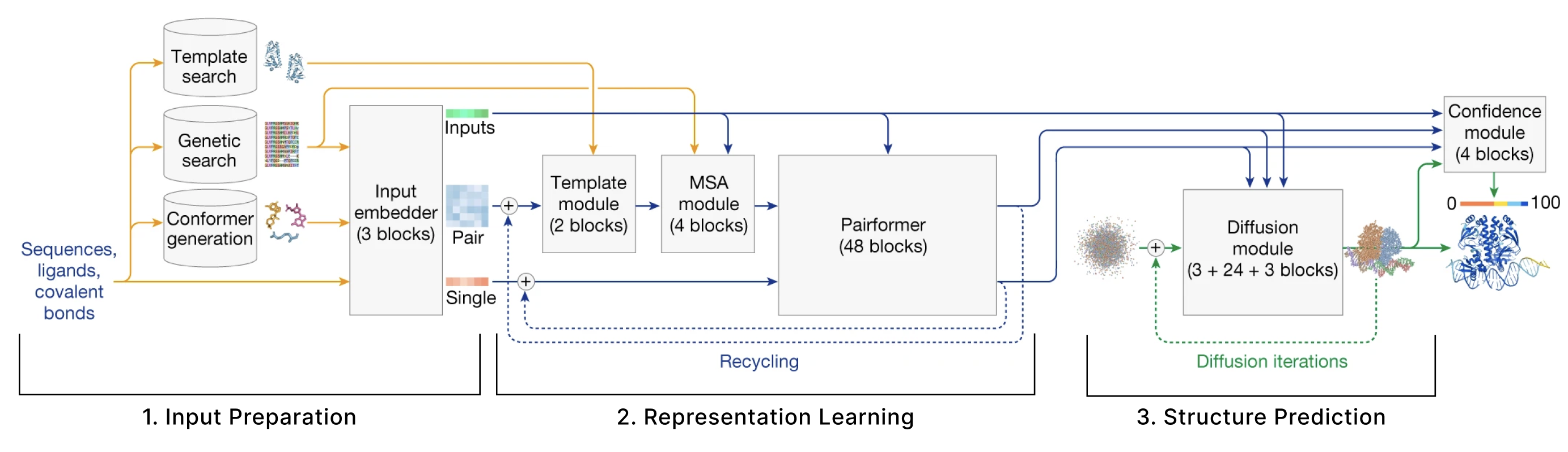
The model can be broken down into 3 main sections:

1. Input Preparation The user provides sequences of some molecules to predict structures for and these need to be embedded into numerical tensors. Furthermore, the model retrieves a collection of other molecules that are presumed to have similar structures to the user-provided molecules. The input preparation step identifies these molecules and also embeds these as their own tensors.
2. Representation learning Given the Single and Pair tensors created in section 1, we use many variants of attention to update these representations.
3. Structure prediction We use these improved representations, and the original inputs created in section 1 to predict the structure using conditional diffusion.

Skip to a specific section by via its name here or the by clicking the relevant part of the architecture in the diagram above.

We also have additional sections describing 4. the loss function, confidence heads, and other relevant training details and 5. some thoughts on the model from an ML trends perspective.

Notes on the variables and diagrams

Throughout the model a protein complex is represented in two primary forms: the “single” representation which represents all the tokens in our protein complex, and a “pair” representation which represents the relationships (e.g. distance, potential interactions) between all pairs of amino acids / atoms in the complex. Each of these can be represented at an atom-level or a token-level, and will always be shown with these names (as established in the AF3 paper) and colors:

• The diagrams abstract away the model weights and only visualize how the shapes of activations change
• The activation tensors are always labeled with the dimension names used in the paper and the sizes of the diagrams vaguely aim to follow when these dimensions grow/shrink. The hidden dimension names usually start with "c" for "channel". For reference the main dimensions used are c_z=128, c_m=64, c_atom=128, c_atompair=16, c_token=768, c_s=384.
• Whenever possible, the names above the tensors in this (and every) diagram match the names of the tensors use in the AF3 supplement. Typically, a tensor maintains its name as it goes through the model. However, in some cases, we use different names to distinguish between versions of a tensor at different stages of processing. For example, in the atom-level single representation, c represents the initial atom-level single representation while q represents the updated version of this representation as it progresses through the Atom Transformer.
• We also ignore most of the LayerNorms for simplicity but they are used everywhere.

---

1. Input Preparation

The actual input a user provides to AF3 is the sequence of one protein and optionally additional molecules. The goal of this section is to convert these sequences into a series of 6 tensors that will be used as the input to the main trunk of the model as outlined in this diagram. These tensors are s, our token-level single representation, z, our token-level pair representation, q, our atom-level single representation, p, our atom-level pair representation, m, our MSA representation, and t, our template representation.

This section contains:

• Tokenization describes how molecules are tokenized and clarifyies the difference between atom-level and token-level
• Retrieval (Create MSA and Templates) expalains why and how we include additional inputs to the model. It creates our MSA (m) and structure templates (t).
• Create Atom-Level Representations creates our first atom-level representations q (single) and p (pair) and includes information about generated conformers of the molecules.
• Update Atom-Level Representations (Atom Transformer) is the main “Input Embedder” block, also called the “Atom Transformer”, which gets repreated 3 times and updates the atom-level single representation (q). The building blocks introduced here (Adaptive LayerNorm, Attention with Pair Bias, Conditioned Gating, and Conditioned Transition) are also relevant later in the model.
• Aggregate Atom-Level -> Token-Level takes our atom-level representations (q, p) and aggregates all the atoms that at part of multi-atom tokens to create token-level representations s (single) and z (pair) and includes information from the MSA (m) and any user-provided information about known bonds that involve ligands.

Tokenization

See where this fits into the full architecture

In AF2, as the model only represented proteins with a fixed set of amino acids, each amino acid was represented with its own token. This is maintained in AF3, but additional tokens are also introduced for the additional molecule types that AF3 can handle:

• Standard amino acid: 1 token (as per AF2)
• Standard nucleotide: 1 token
• Non-standard amino acids or nucleotides (methylated nucleotide, amino acid with post-translational modification, etc.): 1 token per atom
• Other molecules: 1 token per atom

As a result, we can think of some tokens (like those for amino acids) as being associated with multiple atoms, while other tokens (like those for an atom in a ligand) are associated with only a single atom. So, while a protein with 35 standard amino acids (likely > 600 atoms) would be represented by 35 tokens, a ligand with 35 atoms would also be represented by 35 tokens.

Retrieval (Create MSA and Templates)

See where this fits into the full architecture

One of the key early steps in AF3 is something akin to Retrieval Augmented Generation RAG in language models. We find similar sequences to our protein and RNA sequences of interest (collected into a multiple sequence alignment, “MSA”), and any structures related to those (called the “templates”), then include them as additional inputs to the model called m and t, respectively.

(Image from AF2)

Why do we want to include MSA and templates?

Versions of the same protein found in different species can be quite structurally and sequentially similar. By aligning these together into a Multiple Sequence Alignment (MSA), we can look at how an individual position in a protein sequence has changed throughout evolution. You can think about an MSA for a given protein as a matrix where each row is the sequence of the analogous protein from a different species. It has been shown that the conservation patterns found along the column of a specific position in the protein can reflect how critical it is for that position to have certain amino acids present, and the relationships between different columns reflect relationships between amino acids (i.e. if two amino acids are physically interacting, the changes in their amino acids will likely be correlated across evolution). Thus, MSAs are often used to enrich representations of single proteins.

Similarly, if any of these proteins have known structures, those are also likely to inform the structure of this protein. Instead of searching for full structures, only individual chains of the proteins are used. This resembles the practice of homology modeling, in which the structure of a query protein is modeled based on templates from known protein structures that are presumed to be similar.

So how are these sequences and structures retrieved?

First, a genetic search is done searching for any protein or RNA chains that resemble any input protein or RNA chains. This does not involve any training and relies upon existing Hidden Markov Model (HMM) based methodsSpecifically, they use jackhmmer, HHBlits, and nhmmer to scan multiple protein databases and RNA databases for relevant hits. Then these sequences are aligned to each other to construct an MSA with N_MSA sequences. As the computational complexity of the model scales with N_MSA they limit this to N_MSA < 2¹⁴. Typically, MSAs are constructed from individual protein chains but, as described in AF-multimer, instead of just concatenating the separate MSAs together into a block diagonal matrix, certain chains from the same species can be 'paired' as described here. This way, the MSA does not have to be as large and sparse, and evolutionary information can be learned about relationships between chains.

Then, for each protein chain, they use another HMM-based method (hmmsearch) to find sequences in the Protein Data Bank (PDB) that resemble the constructed MSA. The highest quality structures are selected and up to 4 of these are sampled to be included as "templates".

The only new part of these retrieval steps compared to AF-multimer is the fact that we now do this retrieval for RNA sequences in addition to protein sequences. Note that this is not traditionally called “retrieval” as the practice of using structural templates to guide protein structure modeling has been common practice in the field of homology modeling long before the term RAG existed. However, even though AlphaFold doesn’t explicitly refer to this process as retrieval, it does quite resemble what has now been popularized as RAG.

How do we represent these templates?

From our template search, we have a 3D structure for each of our templates and information about which tokens are in which chains. First, the euclidean distances between all pairs of tokens in a given template are calculated. For tokens associated with multiple atoms, a representative “center atom” is used to calculate distances. This would be the C_ɑ atom for amino acids and C¹’ atom for standard nucleotides.

Highlighting "center atoms" in single-token building blocks

This generates a N_token x N_token matrix for each template. However, instead of representing each distance as a numerical value, the distances get discretized into a “distogram” (a histogram of distances).Specifically, the values are binned into 38 bins between 3.15A and 50.75A and there's 1 additional bin for any distances bigger than that.

To each distogram, we then append metadata about which chain In molecular complexes, a chain refers to a distinct molecule or part of a molecule. This can be a protein chain (a sequence of amino acids), a DNA or RNA chain (a sequence of nucleotides), or other biomolecules. AlphaFold uses chain information to differentiate between parts of a complex, helping it predict how these parts interact to form the overall structure each token belongs to, whether this token was resolved in the crystal structure, and information about local distances within each amino acid. We then mask out this matrix such that we only look at distances within each chain (e.g., we ignore the distances between chain A and chain B) as they “make no attempt to select templates… to gain information about inter-chain interactions”‘ It is not specified why, but note that while there is no inter-chain interactions in the templates, they do incorporate them the MSA construction. .

Create Atom-Level Representations

See where this fits into the full architecture

To create q, our atom-level single representation, we need to pull all our atom-level features. The first step is to calculate a “reference conformer” for each amino acid, nucleotide, and ligand. While we do not yet know the structure of the entire complex, we have strong priors on the local structures of each individual component. A conformer (short for conformational isomer) is a 3D arrangement of atoms in a molecule that is generated by sampling rotations about single bonds. Each amino acid has a “standard” conformer which is just one of the low-energy conformations this amino acid can exist in, which can be retrieved through a look-up. However, each small molecule requires its own conformation generation. These are generated with RDKit’s ETKDGv3, an algorithm that combines experimental data and torsion angle preferences to produce 3D conformers.

Then we concatenate the information from this conformer (relative location) with each atom’s charge, atomic number, and other identifiers. Matrix c stores this information for all the atoms in our sequencesIn the AF3 supplement, the atom-level matrices (c, and q) are typically referred to in their vector forms (e.g. c_l or c_m), where l and m are used to index atoms.. We then use c to initialize our atom-level pair representation p to store the relative distances between atoms. Because we only know reference distances within each token, we use a mask (v) to ensure this initial distance matrix only represents distances we’ve calculated in the conformer generation. We also include a linear embedding of the inverse square of the distances, add to it a projection of c_l and c_m, and update this with a few more linear layers with residual connectionsThe AF3 paper doesn't really clarify why this additional inverse distance step is performed or contain ablations for their effect of it; so, as with many of the steps we will discuss, we can only assume they were empirically shown to be useful.In the AF3 supplement, the p tensor is typically referred to in its vector form p_l,m (where this represents the relationship between atom l and atom m)..

Finally, we make a copy of our atom-level single representation, calling this copy q. This matrix q is what we will be updating going forward, but c does get saved and used later.

Update Atom-Level Representations (Atom Transformer)

See where this fits into the full architecture

Having generated q (representation of all the atoms) and p (representation of each pair of atoms), we now want to update these representations based on other atoms nearby. Anytime AF3 applies attention at the atom-level, we use a module called the Atom Transformer. The atom transformer is a series of blocks that use attention to update q using both p and the original representation of q called c. As c does not get updated by the Attention Transformer, it can be thought of as a residual connection to the starting representation.

The Atom Transformer mostly follows a standard transformer structure using layer norm, attention, then an MLP transition. However, each step has been adapted to include additional input from c and p (including a secondary input here is sometimes referred to as “conditioning”.) There is also a ‘gating’ step between the attention and MLP blocks. Going through each of these 4 steps in more detail:

1. Adaptive LayerNorm

Adaptive LayerNorm (AdaNorm) is a variant of LayerNorm with one simple extension. Recall that for a given input matrix, traditional LayerNorm learns two parameters (a scaling factor gamma and a bias factor beta) that adjust the mean and standard deviation of each of the channels in our matrix. Instead of learning fixed parameters for gamma and beta, AdaNorm learns a function to generate gamma and beta adaptively based on the input matrix. However, instead of generating the parameters based on the input getting re-scaled (in the Atom Transformer this is q), a secondary input (c in the Atom Transformer) is used to predict the gamma and beta that re-scale the mean and standard deviation of q.

2. Attention with Pair Bias

Atom-Level Attention with Pair-Bias can be thought of as an extension of self-attention. Like in self-attention, the queries, keys, and values all come from the same 1D sequence (our single representation, q). However, there are 3 differences:

1. Pair-biasing: after the dot product of the queries and keys are calculated, a linear projection of the pair representation is added as a bias to scale the attention weights. Note that this operation does not involve any information from q being used to update p, just one way flow from the pair representation to q. The reasoning for this is that atoms that have a stronger pairwise relationship should attend to each other more strongly and p is effectively already encoding an attention map.

2. Gating: In addition to the queries, keys, and values, we create an additional projection of q that is passed through a sigmoid, to squash the values between 0 and 1. Our output is multiplied by this “gate” right before all the heads are re-combined. This effectively forces the model to ignore some of what it learned in this attention process. This type of gating appears frequently in AF3 and is discussed more in the ML-musings section. To briefly elaborate, because the model is constantly adding the outputs of each section to the residual stream, this gating mechanism can be thought of as the model’s way to specify what information does or does not get saved in this residual stream. It is presumably named a “gate” after the similar “gates” in LSTM which uses a sigmoid to learn a filter for what inputs get added to the running cell state.

3. Sparse attention:

Because the number of atoms can be much larger than the number of tokens, we do not run full attention at this step, rather, we use a type of sparse attention (called Sequence-local atom attention) in which the attention is effectively run in local groups where groups of 32 atoms at a time can all attend to 128 other atoms. Sparse attention patterns are more thoroughly described elsewhere on the internet.

3. Conditioned Gating

We apply another gate to our data, but this time the gate is generated from our origin atom-level single matrix, cAs with so many steps, it is unclear why it is done this way and what the benefit of conditioning on the original representation c does as opposed to learning the gate from the primary single representation q.

4. Conditioned Transition

This step is equivalent to the MLP layers in a transformer, and is called “conditioned” because the MLP is sandwiched in between Adaptive LayerNorm (Step 1 of Atom Transformer) and Conditional Gating (Step 3 of Atom Transformer) which both depend on c.

The only other piece of note in this section is that AF3 uses SwiGLU in the transition block instead of ReLU. The switch from ReLU → SwiGLU happened with AF2 → AF3 and has been a common change in many recent architectures so we visualize it here.

With a ReLU-based transition layer (as in AF2), we take the activations, project them up to 4x the size, apply a ReLU, then down-project them back to their original size. When using SwiGLU (in AF3), the input activation creates two intermediate up-projections, one of which goes through a swish non-linearity (improved variant of ReLU), then these are multiplied before down-projecting. The diagram below shows the differences:

Aggregate Atom-Level → Token-Level

See where this fits into the full architecture

While the data so far has all been stored at an atom-level, the representation learning section of AF3 from here onwards operates at the token-level. To create these token-level representations, we first project our atom-level representation to a larger dimension (c_atom=128, c_token=384). Then, we take the mean over all atoms assigned to the same token. Note that this only applies to the atoms associated with standard amino acids and nucleotides (by taking the mean across all atoms attached to the same token), while the rest remain unchangedThe AF3 paper describes these molecule types as having a representative atom per token (the center atom). Recall that this is the C_α atom for amino acids and C¹' atom for standard nucleotides. So while we mostly consider this reduced representation as "token space", we can also think of each token as representing a single atom (either a representative C_α/C¹' atom or an individual atom)..

Now that we are working in “token space”, we concatenate our token-level features and statistics from our MSA (where available)e.g., The amino acid type (dim = 32), distribution of amino acids at this position in our MSA (dim = 32), and the deletion mean at this token (dim = 1) from our MSA. Note that these values will be zero for ligand atoms not associated with an MSA.. This matrix, s^inputs, having grown a bit from these concatenations, is projected back down to c_token, and called s^init: the starting representation of our sequence that will be updated in the representation learning section. Note that s^init gets updated in the representation learning section, but s^inputs are saved to be used later in the structure prediction section.

Now that we have created s^init, our initialized single representation, the next step is to initialize our pair representation z^init. The pair representation is a three dimensional tensor, but it’s easiest to think of it as a heatmap-like 2D matrix with an implicit depth dimension of c_z=128 channels. So, entry z_i,j of our pair representation is a c_z dimensional vector meant to store information about the relationship between token i and token j in our token sequence. We have created an analogous atom-level matrix p, and we follow a similar process here at the token-level.

To initialize z_i,j, we use a linear projection to make the channel dimension of our sequence representation match that of the pair representation (384 → 128) and add the resulting s_i and s_j. To this, we add a relative positional encoding, p_i,jThis encoding consists of a^rel_pos, a one-hot encoding of the offset of the two token ids in token space (or set to a maximum of 65 if the two tokens are not on the same chain), a^rel_token, a one-hot encoding of the offset of the two token ids in token space (or set to a maximum of 65 if the tokens are part of different amino acids or nucleotides), and a^rel_chain, encoding the offset of the two chains the tokens are on. We project this concatenated encoding into the dimensionality of z too.. If the user has also specified particular bonds between tokens, those are linearly embedded here and added to that entry in the pair representation.

Now we’ve successfully created and embedded all of the inputs that will be used in the rest of our model:

For Step 2, we will set aside the atom-level representations (c, q, p) and focus on updating our token-level representations s and z in the next section (with the help of m and t).

2. Representation Learning

(Diagram modified from full AF3 architecture diagram)

This section is the majority of the model, often referred to as the “trunk”, as it is where most of the computation is done. We call it the representation learning section of the model, as the goal is to learn improved representations of our token-level “single” (s) and “pair” (z) tensors initialized above. Recall that we refer to the "single" sequence representations, these are not necessarily the sequence of one protein, but rather the concatenated sequence of all the atoms or tokens in our structure (which could contain multiple separate molecules).

This section contains:

1. Template module updates z using the structure templates t
2. MSA module first updates the MSA m, then adds it to the token-level pair representation z. In this section we spend significant time on two operations:
   • The Outer Product Mean enables m to influence z
   • MSA Row-wise Gated Self-Attention Using Only Pair Bias updates m based on z and is a simplified version of attention with pair-bias (intended for MSAs)
3. Pairformer updates s and z with geometry-inspired (triangle) attention. This section mostly describes the triangle operations (used extensively throughout both AF2 and AF3).
   • Why look at triangles? explains some intuition for the triangle operations
   • Triangle Updates and Triangle Attention both update z using methods similar to self-attention, but inspired by the triangle inequality
   • Single Attention With Pair Bias updates s based on z and is the token-level equivalent of attention with pair-bias (intended for single sequences)

Each individual block is repeated multiple times, and then the output of the whole section is fed back into itself again as input and the process is repeated (this is called recycling).

Template Module

See where this fits into the full architecture

Each template (N_templates=2 in the diagram) goes through a linear projection and is added together with a linear projection of our pair representation (z). This newly combined matrix goes through a series of operations called the Pairformer Stack (described in depth later). Finally, all of the templates are averaged together and go through - you guessed it - another linear layer.This is both called the template module and template embedder depending on where you look in the AF3 supplement, but they seem to just refer to the same thing. Interestingly, this last linear layer has a ReLU as the non-linearity which wouldn’t be particularly notable except for the fact that it is one of only two places ReLU is used as the non-linearity in AF3. As always, can only hypothesize as to why this was selected.

MSA Module

See where this fits into the full architecture

Architecture of MSA Module. {Diagram from AF3}

This module greatly resembles what was called “Evoformer” in AF2, and the goal of it is to simultaneously improve the MSA and pair representations. It does a series of operations independently on these two representations then also enables cross-talk between them.

The first step is to subsample the rows of the MSA, rather than use all rows of the MSA previously generated (which could be up to 16k), then add a projected version of our single representation to this subsampled MSA.

Outer Product Mean

Next, we take the MSA representation and incorporate it into the pair representation via the “Outer Product Mean”. Comparing two columns of the MSA reveals information about the relationships between two positions in the sequence (e.g. how correlated are these two positions in the sequence across evolution). For each pair of token indices i,j, we iterate over all evolutionary sequences, taking the outer product of m_s,i and m_s,j, then averaging these across all the evolutionary sequences. We then flatten this outer product, project it back down, and add this to the pair representation z_i,j (full details in diagram). While each outer product only compares values within a given sequence m_s, when we take the mean of these, that mixes information across sequences. This is the only point in the model where information is shared across evolutionary sequences. This is a significant change to reduce the computational complexity of the Evoformer in AF2.

Row-wise gated self-attention using only pair bias

Having updated the pair representation based on the MSA, the model next updates the MSA based on the pair representation. This specific update pattern is called row-wise gated self attention using only pair bias, and is a simplified version of self attention with pair bias, discussed in the Atom Transformer section, applied to every sequence (row) in the MSA independently. It is inspired by attention, but instead of using queries and keys to determine what other positions each token should attend to, we just use the existing relationships between tokens stored in our pair representation z.

In the pair representation, each z_i,j is a vector containing information about the relationship between tokens i and j. When the tensor z gets projected down to a matrix, each z_i,j vector becomes a scalar that can be used to determine how much token i should attend to token j. After applying row-wise softmax, these are now equivalent to attention scores, which are used to create a weighted average of the values as a typical attention map would.

Note that there is no information shared across the evolutionary sequences in the MSA as it is run independently for each row.

Updates to pair representation

The last step of the MSA module is to update the pair representation through a series of steps referred to as triangle updates and attention. These triangle operations are described below with Pairformer, where they are used again. There are also some transition blocks that use SwiGLU to up/down project the matrix as was done in the Atom Transformer.

Pairformer module

See where this fits into the full architecture

Diagram from AF3 supplement

Having updated our pair representation based on the templates and MSA Module, we now ignore them for the rest of the model. Instead, only the updated pair representation (z) and single representation (s) enter the Pairformer and are used to update each other. As the transition blocks have already been described, this section focuses on the Triangle Updates and Triangle Attention, then briefly explains how the Single Attention with Pair Bias differs from the variant described earlier. These triangle-based layers were first introduced in AF2 are one of the pieces that not only remained in AF3, but now are even more present in the architecture, so they get quite a bit of attention.

Why look at triangles?

The guiding principle here is the idea of the triangle inequality: “the sum of any two sides of a triangle is greater than or equal to the third side”. Recall that each z_i,j in the pair tensor encodes the relationship between positions i and j in the sequence. While it does not literally encode the physical distances between pairs of tokens, let’s think about it for a moment as if it did. If we imagine that each z_i,j is the distance between two amino acids and we know z_i,j=1 and z_j,k=1. By the triangle inequality z_i,k cannot be larger than \(\sqrt{2}\). Knowing two of the distances gives us a strong belief about what the third distance must be. The goal of triangle updates and triangle attention are to try to encode these geometric constraints into the model.

The triangle inequality is not enforced in the model but rather, it is encouraged through ensuring each position z_i,j is updated by looking at all possible triplets of positions (i,j,k) at a time. So z_i,j is updated based on z_j,k and z_i,k for all other atoms k. Because z represents the complex physical relationship between these tokens, rather than merely their distance, these relationships can be directional. So for z_i,j, we also want to encourage consistency with z_k,i and z_k,j for all atoms k. If we think of the atoms as a graph, with z as a directed adjacency matrix, it makes sense that AlphaFold calls these “outgoing edges” and “incoming edges”.

Consider row i=0 of this adjacency matrix, and let’s say we want to update z_0,2, which has been highlighted in purple. The idea behind the update is that if we know the distances between 0→1 and 2→1, that gives us some constraints on what 0→2 can be. Similarly, if we know the distances between 0→3 and 2→3, this also gives us a constraint on 0→2. This would apply for all atoms k.

So, in the triangle updates and attention, we effectively look at all directed paths for 3 nodes in this graph (a.k.a triangles, hence the name!).

Triangle Updates

Having carefully looked at the triangle operations from a graph theory perspective, we can see how this is implemented with tensor operations. In the outgoing update, every position z_i,j in the pair representation gets updated independently based on a weighted combination of the other elements in the same row (z_i,j), where the weighting of each z_i,k is based on the third element in its outgoing edge triangle (z_j,k).

Practically, we take three linear projections of z (called a, b, and g). To update z_i,j, we take an element-wise multiplication of row i from a and row j from b. We then sum over all these rows (different values of k), and gate with our g projection.

At this point you might notice that gating is used all throughout this architecture!

For the incoming update, we effectively do the same thing but flipping the rows with the columns, so to update z_i,j we take a weighted sum of the other elements in the same column (z_k,j), where the weighting of each z_k,j is based on the third element in its outgoing edge triangle (z_k,i). After creating the same linear projections, we take an element-wise multiplication of column i from a and column j from b, and sum over all the rows of this matrix. You’ll find that these operations exactly mirror the graph-theory adjacency view described above.

Triangle Attention

After our two triangle update steps, we also update each z_i,j using triangle attention for the outgoing edges and triangle attention for the incoming edges. The AF3 paper refers to the “outgoing edges” as attention “around starting node” and “incoming edges” as attention “around ending node”.

To build up to triangle attention, it can be helpful to start with typical self-attention over a 1D sequence. Recall that queries, keys, and values are all transformations of the original 1D sequence. An attention variant called axial attention extends this to matrices by applying independent 1D self-attention over the different axes of a 2D matrix (the rows, then the columns). Triangle attention adds the triangle principle we discussed earlier to this, updating z_i,j by incorporating z_i,k and z_j,k for all atoms k. Specifically, in the “starting node” case, to calculate the attention scores along row i (to determine how much z_i,j should be influenced by z_i,k), we do a query-key comparison between z_i,j and z_i,k as usual, then bias the attention based on z_j,k as is shown above.

For the “ending node” case, we again swap rows for columns. For z_i,j, the keys and values will both come from column i of z, while the bias will come from column j. So, when comparing the query z_i,j with the key z_k,i, we bias that attention score based on z_k,j. Then, once we have attention scores over all k, we use our values vectors from column i.

Single Attention with Pair Bias

Now that we’ve updated our pair representation with these four triangle steps, we pass the pair representation through a Transition block as described above. Finally, we want to update our single representation (s) using this new updated pair representation (z), so we will use single attention with pair bias, pictured below. This is identical to Single Attention with Pair Bias describedFor reference, in the AF3 supplement, Single Attention with Pair Bias is also referred to as "Attention Pair Bias" in the Atom Transformer section, but at the token-level. As it operates on the token-level, it uses full attention as opposed to the block-wise sparse pattern used when operating at the atom-level.

We repeat the Pairformer for 48 blocks, eventually creating s^trunk and z^trunk.

3. Structure Prediction

Basics of Diffusion

Now, with these refined representations, we are ready to use s and z to predict the structure of our complex. One of the changes introduced in AF3 is that entire structure prediction is based on atom-level diffusion. Existing posts more thoroughly explain the intuition and math for diffusion, but the basic idea of a Diffusion Model is to start with real data, add random noise to your data, then train a model to predict what noise was added. Noise is iteratively added to the data over a series of T timesteps to create a sequence of T variants of each datapoint. We call the original data point x_t=0 and the fully noised version x_t=T. During training, at timestep t, the model is given the x_t and predicts what noise was added between x_t-1 and x_t. We take a gradient step on the predicted noise added compared to the actual noise that had been added.

Then, at inference time, we simply start with random noise, which is equivalent to x_t=T. For every time step, we predict the noise the model thinks has been added, and remove that predicted noise. After a pre-specified number of timesteps, we end up with a fully “denoised” datapoint that should resemble the original data from our dataset.

Conditional Diffusion lets the model ‘condition’ these de-noising predictions on some input. Practically this means that for each step of the model, it takes three inputs:

1. The current noisy iteration of our generation
2. A representation of the current time step we are at
3. The information we want to condition on (this could be a caption for an image to generate, or properties for a protein).

As a result, the final generation is not just a random example that resembles the training data distribution, but should specifically match the information represented by this conditioning vector.

With AF3, the data we learn to de-noise is a matrix x with the x,y,z coordinates of all the atoms in our sequences. During training, we add Gaussian noise to these coordinates until they are effectively fully random. Then at inference time, we start with random coordinates. At each time step, we first randomly rotate and translate our entire predicted complex. This data-augmentation teaches the model that any rotation and translation of our complex is equally valid, and replaces the much more complicated Invariant Point Attention used in AF2. AF2 had developed a complicated architecture called Invariant Point Attention meant to enforce equivariance to translations and rotations. This led to a vigorous debate over the importance of IPA in AF2's success. In AF3, this is dropped in favor of a much simpler approach: applying random rotations and translations as data-augmentations to help the model learn such equivariances naturally. So here we simply randomly rotate all atoms' coordinates around the center of our current generation (the mean over all atoms' coordinates), and randomly sample a translation in each dimension (x, y, and z) from a N(0,1) Gaussian. It appears from the algorithm that the translation is universal, that is the same translation is applied to every atom in our current generation. This type of data augmentation was popularize with CNNs but in the past few years, equivariant architectures like IPA have been considered an more efficient and elegant approach to solve the same problem. Thus, when AF3 replaced equivariant attention with data-augmentation, it sparked a lot of internet discussions. We then add a small amount of noise to the coordinates to encourage more heterogeneous generations.It benefits us for the model to generate several slightly different variations. At inference time, we can score each using our confidence head, and return only the generation with the highest score. Finally, we predict a de-noising step using the Diffusion Module. We cover this module in more detail below:

Data (coordinates) to get de-noised

Diffusion Module

See where this fits into the full architecture

In each de-noising diffusion step, we condition our prediction on multiple representations of the input sequences:

• the outputs of the trunk (our post-Pairformer updated s and z, now called s^trunk and z^trunk)
• the initial atom and token-level representations of the sequence created in the input embedder that have not gone through the trunk (s^inputs, c^inputs)

The AF3 paper breaks down its diffusion process into 4 steps that involve moving from tokens to atoms, back to tokens, and back to atoms:

1. Prepare token-level conditioning tensors
2. Prepare atom-level conditioning tensors, update them using the Atom Transformer, and aggregate them back to token-level
3. Apply attention at the token-level, and project back to atoms
4. Apply attention at the atom-level to predict atom-level noise updates

1. Prepare token-level conditioning tensors

To initialize our token-level conditioning representation, we concatenate z^trunk to the relative positional encodings then project this larger representation back down and pass it through several residual-connection transition blocks.

Similarly, for our token-level single representation, we concatenate the very first representation of the input created at the start of the model (s^inputs) and our current representation (s^trunk), then project it back down to its original size. We then create a Fourier embedding based on the current diffusion time stepMore specifically, the amount of noise associated with this timestep in the Noise Schedule, add that to our single representation, and pass that combination through several Transition blocks. By including the diffusion time step in the conditioning input here, it ensures the model is aware of the timestep in the diffusion process when making de-noising predictions, and so predicts the right scale of noise to remove for this timestep.

2. Prepare atom-level tensors, apply atom-level attention, and aggregate back to token-level

At this point, our conditioning vectors are storing information at a per-token level, but we want to also run attention at the atom-level. To address this, we take our initial atom-level representations of the input created in the Embedding section (c and p), and update them based on the current token-level representations, to create atom-level conditioning tensors.

Next, we scale the atom’s current coordinates (x) by the variance of the data, effectively creating “dimensionless” coordinates with unit variance (called r). We then update q based on r such that q is now aware of the atom’s current location. Finally, we update q with the Atom Transformer (which also takes the pair representation as input), and aggregate the atoms back to tokens as we’ve previously seen.Recall from the input preparation section that Atom Transformer runs sparse attention over the atoms, and all steps (layer norm, attention, gating) are conditioned on the conditioning tensor c.

At the end of this step, we return

• q: updated atom representation after incorporating information about the atom’s current coordinates
• a: token-level aggregated form of q, capturing coordinates and sequence information
• c: atom representation for conditioning based on the trunk
• p: our updated atom-pair representation for conditioning

3. Apply attention at the token-level

The goal of this step is to apply attention to update our token-level representation of the atom coordinates and sequence information, a. This step uses the Diffusion Transformer visualized during input preparation, which mirrors the Atom Transformer but for tokens.

4. Apply attention at the atom-level to predict atom-level noise updates

Now, we return to atom space. We use our updated a (token-level representations based on current “center atom” locations) to update q (atom-level representation of all atoms based on current location) using the Atom Transformer. As was done in step 3, we broadcast our tokens representation to match the number of atoms we started with (selectively duplicating the tokens that represent multiple atoms), and run the Atom Transformer. Most importantly, one last linear layer maps this atom-level representation q back to R³. This is the key step: we’ve used all these conditioning representations to generate coordinate updates r^update for all atoms. Now, because we generated these in the “dimensionless” space r_l, we carefully re-scaleThis careful scaling involves both the variance of our data, and the noise schedule based on our current timestep, so that our updates are smaller and smaller as we get deeper into the de-noising process. the updates from r^update to their form with non-unit variance, x^update, and apply the updates to x_l.

With that, we’ve completed our tour through the main architecture of AlphaFold 3! Now we provide some additional information about the loss function, auxiliary confidence heads, and training details.

4. Loss Function and Other Training Details

Loss function and confidence heads

\(L_{\text{loss}} = L_{\text{distogram}}*\alpha_{\text{distogram}}+L_{\text{diffusion}}*\alpha_{\text{diffusion}}+L_{\text{confidence}}*\alpha_{\text{confidence}}\)

The loss is a weighted sum of 3 terms:

• L_distogram which evaluates the accuracy of the predicted distogram at a token-level
• L_diffusion which evaluates the accuracy of the predicted distogram at an atom-level. It looks at all pairwise distances then includes additional terms to prioritize distances between nearby atoms and atoms involved in protein-ligand bonds.
• L_confidence which evaluates the model’s self-awareness about which structures are likely to be inaccurate

L_distogram

The output of our model is atom-level coordinates, which can easily be used to create an atom-level distogramRecall how the distograms were initially created by binning pairwise distances between atoms. However, this loss evaluates a token-level distogram. To get the xyz coordinates for tokens, we just use the coordinate of the “center atom”. As these distogram distances are categorical, the predicted distogram is then compared to the true distogram via cross entropy.

L_diffusion

The diffusion loss itself is a weighted sum of three terms each computed over the atom positions, additionally scaled by the amount of noiset^{^}, the sampled noise level for the current time step, and σ_data, the variance of the data which scales the amount of noise at each time step added at the current time step: \(L_{\text{diffusion}} = (L_{\text{MSE}} + L_{\text{bond}} * \alpha_{\text{bond}}) * (\hat{t}^2 + \sigma_{\text{data}}^2)/(\hat{t}+\sigma_{\text{data}})^2 + L_{\text{smooth_lddt}}\)

• L_MSE is a version of the distogram loss we just discussed, but over all atoms rather just “center atoms” (and with DNA, RNA, and ligand atoms upweighted). Additionally, it looks at the mean squared error between positions, rather than binning them into a distogram.
• L_bond aims to ensure the accuracy of bond lengths for protein-ligand bonds by adding an additional MSE loss on the difference in predicted and ground-truth distograms for atom-pairs that are part of protein-ligand bonds.There are various stages of training and α_bond is set to 0 in the initial stages, so this term is only introduced later.
• L_{smooth_LDDT} (smoothed local distance difference test) is yet another variant of the distogram loss that tries to capture the accuracy of local distances. An atom-pair’s predicted distance “passes the test” if it is within a given threshold of the atom-pair’s true distance. To make this metric smooth and differentiable, we pass the difference between predicted and ground-truth distograms through a sigmoid centered on the test’s threshold. We can think of this as generating a probability (between 0 and 1) that this atom-pair passes the test. We take the average of four “tests’’ with increasingly tight thresholds (4, 2, 1, and .5 Å). Using this loss encourages the model to reduce the probability of failing each test. Finally, to make the test “local”, we ignore the loss for an atom-pair if that atom-pair’s ground truth distance is large, as we only want the model to focus on accurately predicting an atom’s distances to nearby atomsSpecifically, for an atom-pair l,m, we ignore the loss for l and m if l and m are more than 30 Å away if atom m is part of a nucleotide. We ignore the loss for l and m if they are more than 15 Å away from each other and m is not a nucleotide (so is part of a protein or ligand)..

L_confidence

The goal of this loss is not to improve the accuracy of the structure, but rather to teach the model to predict its own accuracy. This loss is a weighted sum of 4 terms that each correspond to a method of evaluating the quality of a predicted structure:

\[L_{\text{confience}} = L_{\text{plDDT}} + L_{\text{PDE}} + L_{\text{resolved}} + L_{\text{PAE}} * \alpha_{\text{PAE}}\]

• lDDT Atom-level “local distance difference test”, capturing the expected accuracy of an atom’s predicted distances to nearby atoms.

• PAE Predicted alignment error between token i’s predicted and the ground-truth positions. We first rotate and translate the predicted token i and ground-truth token i into the frame of token j. That is, if we assume for a moment token j is in exactly its ground-truth position, we predict how close token i is to where it should be, based on its relation to token j.

• PDE Predicted distance error between tokens, capturing the accuracy of predicted differences between all pairs of tokens.

• Experimentally resolved prediction The model predicts which atoms were experimentally resolved (not every atom is experimentally resolved in every crystal structure).

To get these confidence losses for each of the metrics, AF3 predicts values for these error metrics, then these error metrics are calculated on the predicted structure, and the loss is based on the difference between these two. So even if the structure is really incorrect and the PAE is high, if the predicted PAE is also high, the L_pae will be low.

These confidence predictions are generated mid-way through the diffusion process. At a selected diffusion step t, the predicted coordinates r^t are used to update the single and pair representations created in the representation learning trunk. The predicted errors are then calculated from linear projections of the updated pair representation (for PAE and PDE) or this updated single representation (pLDDT and experimentally resolved). Then, the actual error metrics are calculated based on the same generated atom coordinates (process described below, if interested) for comparison.

While these terms are included in the confidence head loss, gradients from these terms are only used to update the confidence prediction heads and do not affect the rest of the model.

How are the actual error metrics calculated?

pLDDT: The LDDT for atom l is calculated in the following way: in the current predicted structure, we calculate the distance between atom l and a set of atoms R that is indexed by m, and compare this to the ground truth equivalent. To be in this set, an atom m must be part of a polymer chain, within 15 or 30 Å of l depending on the molecule m is a part of, and the center atom of a token. We then calculate four binary distance tests with increasingly tight thresholds (4, 2, 1, and .5 Å) and take the average pass rate, and sum over the atoms in R. We bin this percentage into 50 bins between 0 and 1.

At inference time, we have a pLDDT head. This head takes the single representation of a given token, repeats it out across all the atoms "attached" to this tokenTechnically, the max number of atoms attached to any token, so that we can stack tensors, and projects all those atom-level representations to the 50 bins of our pLDDT_l. We treat these as logits across the 50 "classes", use a softmax to convert to probabilities, and take a multi-class classification loss across the bins.

Predicted Alignment Error (PAE): Every token is considered to have a frame, that is a 3D coordinate frame created from three atoms (called a, b, c) involved in that token. Atom b within those three atoms forms the origin in this frame. In cases where each token has a single atom "attached", the center atom of the frame is the single atom of the token, and the two other nearest tokens of the same entity (e.g., same ligand) form the basis of the frame. For every token pair (i,j) we re-express the predicted coordinates of the center atom for token_i using the frame of token_j. We do the same for the ground-truth coordinates of the center atom of token_i. The euclidean distance between these transformed true and predicted coordinates of the center atom of token_i is our alignment error, binned into 64 bins. We predict this alignment error from the pair representation z_i,j, projecting it to 64 dimensions that we treat as logits and convert to probabilities with a softmax. We train this head with a classification loss, which each bin as a class. See here for additional details.

Third, AF3 predicts the distance error (PDE) between tokens. The true distance error is calculated by taking the distance between center atoms for every token pair, and binning these distances over 64 uniformly-sized bins from 0 Å to 32 Å. The predicted distance error comes from projecting the pair representation z_i,j plus the pair representation z_j,i into 64 dimensions that we again treat as logits, and again convert to probabilities with a softmax.

Finally, AF3 predicts whether each atom was experimentally resolved in the ground-truth structure. Similar to the pLDDT head, we repeat the s_i single representation out for the number of atoms this token represents, and project to 2 dimensions and use a binary classification loss.

---

Other Training Details

Now that the architecture is covered, the last pieces are some of the additional training details.

Recycling

As introduced in AF2, AF3 recycles its weights; that is, rather than making the model deeper, the model weights are re-used and inputs are run through the modules multiple times to continually improve the representations. Diffusion inherently uses recycling at inference time, as the model is trained to incorporate the timestep information and use the same model weights for every time step.

Cross-distillation

AF3 uses a mix of synthetic training data generated by itself (via self-distillation) but also by AF2, via cross-distillation. Specifically, the authors note that, by switching to the diffusion-based generative module, the model stopped producing the characteristic “spaghetti” regions that allowed users of AF2 to visually identify low-confidence and likely disordered regions. Just visually looking at the diffusion-based generations, all regions appeared equally high in confidence, making it more difficult to identify potential hallucinations.

To solve this problem, they included generations from AF2 and AF-Multimer in the training data for AF3, allowing the model to learn that, when AF2 was not confident in its prediction, it should output these unfolded regions and to “instruct” AF3 to do the same.Nucleic acids and small molecules in distillation datasets had to be removed as they could not be processed by AF2 and AF-multimer. However, once previous models generated new predicted structures, and these structures got aligned to the originals, the removed molecules were added back in. If adding these back in created new atom clashes, the whole structure was excluded, to avoid accidentally teaching the model to accept clashes.

(Diagram from AF3 paper)

Cropping and Training Stages

While no part of the model has an explicit restriction on the length of the input sequences, the memory and compute requirements increase significantly with sequence length (recall the multiple O(N_tokens³ operations)). Thus, for efficiency the proteins get randomly cropped. As introduced in AF-multimer, because we want to model the interactions between multiple chains, the random cropping needs to include all of these. They use 3 methods for cropping and all 3 of these are used in different proportions depending on the training data (ex: PDB crystal structure vs disordered PDB complex vs distillation, etc.)

• Contiguous cropping: Contiguous sequences of amino acids are selected for each chain
• Spatial cropping: Amino acids are selected based on distance to a reference atom (typically this atom is part of a specific chain or binding interface of interest)
• Spatial interface cropping: Similar to spatial cropping, but based on distances to atoms that specifically at a binding interface.

While a model trained on random crops of 384 can be applied to longer sequences, to improve the model’s ability to handle these sequences, it is iteratively fine-tuned on larger sequence lengths. The mix of datasets and other training details is also varied in each training stage as is shown in the table below.

(Table from AF3 supplement)

Clashing

The authors note that AF3’s loss does not include a clash penalty for overlapping atoms. While switching to a diffusion-based structure module means the model could in theory predict two atoms to be in the same location, this seems to be minimal after training. That said, AF3 does employ a clashing penalty when ranking generated structures.

Batch sizes

Although the diffusion process sounds quite involved, it is still significantly less computationally expensive than the trunk of the model. Thus, the AF3 authors found that it is more efficient from a training perspective to expand the batch size of the model after the trunk. So for each input structure, it gets run through the embedding and trunk, then 48 independent data-augmented versions of the structure are applied, and these 48 structures are all trained in parallel.

That’s it for the training process! There are some other small details but this is probably already more than you need, and if you’ve made it this far, the rest should be easy to pick up from reading the AF3 supplement.

ML Musings

Having walked so thoroughly through the architecture of AF3 and its comparisons to AF2, it is interesting how the choices made by the authors fit into broader Machine Learning trends.

AlphaFold as Retrieval-Augmented Generation

At the time AF2 was released, it was not common to include retrievals from the training set at inference time. In the case of AF, utilizing an MSA and template search. MSA-based methods were being used for protein modeling, but this type of retrieval was less used in other areas of Deep Learning (i.e., ResNets do not embed relevant training images at inference time when classifying a new image in Computer Vision, for example). Although AF3 reduces the emphasis on the MSA compared to AF2 (it is no longer operated on and updated in the 48 blocks of the Evoformer/Pairformer), they still incorporate both the MSA and templates, even as other protein prediction models such as ESMFold have dropped retrieval in favor of fully parametric inference.

Interestingly, some of the largest and most successful Deep Learning models now often include similar additional information at inference time. While the details of the retrieval systems are not always disclosed, Large Language Models routinely use Retrieval Augmented Generation systems such as a traditional web search at inference time to orient the model toward relevant information (even if that information was likely already in its training data) that should guide inference. It will be interesting to see how the use of directly relevant examples at inference time develops in the future.

Pair-Bias Attention

One of the major components of AF2 that is even more present in AF3 is Pair-Bias Attention. That is, attention where the queries, keys, and values all originate from the same source (like in self-attention), but where there is a bias term added to the attention map from another source. This effectively acts as a light-touch version of information sharing, without full cross-attention. Pair-Bias Attention appears in almost every module. While this type of attention is now used in other protein modeling architectures, we have not seen this particular type of cross-biasing used in other fields (although that does not mean it hasn’t been done!). Perhaps it only works well here because the pair-representation is naturally analogous to a self-attention map already, but is an intriguing alternative to pure self or pure cross-attention.

Self-supervised training

Self-supervised models like ESM have been able to achieve impressive results at predicting protein structure by replacing the MSA embedding with a “probabilistic MSA” using self-supervised pre-training. In AF2, the model had an additional task that predicted masked tokens from the MSA, achieving a similar self-supervision, but that was removed with AF3. We have not seen commentary from the authors on why they did not use any self-supervised language modeling pre-training approach on the MSA, and in fact decreased the compute used to process the MSA. Three possible reasons self-supervised learning is not used to initialize the MSA embeddings are 1) they viewed the massive pre-training phase as a suboptimal use of compute 2) they tried it and found that including a small MSA module outperformed pre-trained embeddings and was worth the additional inference-time cost or 3) utilizing a mix of pre-trained embeddings for amino acid tokens and randomly initialized embeddings for DNA/RNA/ligands would not be compatible or underperformed fully supervised training on their hybrid atom-token structure. By focusing on self-supervision tasks, models in the ESM family are also much more simple than AF3 (although they don't handle DNA/RNA/ligands and have slightly different goals.) It is interesting to watch that as some models aim to maximize architectural simplicity, AlphaFold remains this complicated!

Classification vs. Regression

As in AF2, AF3 continues to use a mix of MSE and binned classification losses. The classification components are interesting as, if the model predicts a distogram bin that is only off-by-one, it gets no “credit” for being close rather than way off. It is unclear what informed this design decision, but perhaps the authors found the gradients to be more stable than working with several different MSE losses, and perhaps the per-atom losses saw so many gradient steps that the additional signal from a continuous loss would not have proven beneficial.

Similarities to Recurrent Architectures (e.g LSTMs)

AF3’s architecture incorporates several design elements reminiscent of recurrent neural networks that are not typically found in traditional transformers:

• Extensive Gating: AF3 uses gating mechanisms throughout its architecture to control information flow in the residual stream. This is more akin to the gating in LSTMs or GRUs than the standard feed-forward nature of normal transformer layers.
• Iterative Processing with Weight Reuse: AF3 applies the same weights multiple times to progressively refine its predictions. This process, involving both recycling and the diffusion model, resembles how recurrent networks process sequential data over time steps using a shared set of weights. It differs from standard transformers, which typically make predictions in a single forward pass. This approach allows AF3 to iteratively improve its protein structure predictions without increasing the number of parameters.
• Adaptive Computation: The recycling is also similar to the iterative updating used in diffusion and quite related to the idea of adaptive compute time (ACT), originally introduced to dynamically determine how much compute to use for RNNs and more recently used in Mixture-of-Depths to achieve a similar goal with transformers. This contrasts with the fixed depth of standard transformers and theoretically would allow the model to apply more processing to challenging inputs.

It was shown in the AF2 ablations that the recycling was important, but there was little disucssion on the importance of gating. Presumably it helps with training stability as in LSTMs but it is interesting that it is so prevalent here yet not in many other transformer-based architectures.

Cross-distillation

The use of AF2 generations to re-introduce its distinctive style specifically for low-confidence regions is very interesting. If there is a lesson here, it may be the most practical of all: If your previous model is doing one specific thing better than your new model, you can try cross-distillation to get the best of both worlds!

---

If you’ve made it this far, thanks for reading and hope it was helpful!! If you have any questions / comments / corrections / feedback feel free to reach out to us on twitter (E, J) or email (E, J) !

Special thanks to Kristy Carpenter, Nicholas Joseph, Kyle Swanson, and Kara Liu for giving feedback on this 💜